
Tyres and Artificial Neural Networks – Pt2
In Part 1 we talked about the real tyre, what is a virtual tyre and why use a ANN (Artificial Neural Network) to generate a virtual tyre model. Now is the time to “train” the ANN and then to generate a new virtual tyre model.
ANN TRAINING
An ANN is composed by several basic elements, neurons, that are linked to each other.
Each neuron of the net is made to give a “weight” and a “bias” to each input it receives (fig. 3). 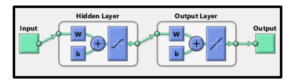
After you have structured and built an ANN, you have to train it. That means you have to feed the ANN with a reasonably high number of data (input & output), on which it can make the Machine Learning process.
Given input and output, the ANN tries to “understand” the correlation between them, making some “attempts”.
After any attempt the ANN adjusts wights and bias of its neurons in order to reach the output- target given. (fig. 4).
At this point your are feeding the machine learning process.
Anytime the ANN repeat the process the generate outputs are getting closer and closer to the output-target given; the ANN cuts down the error margin in an asymptotic way (fig.5).
When the error margin falls within an acceptable range, we can end the machine learning process.
Now our tool is ready to receive brand new inputs and to giveback new outputs.
FUNCTION FITTING PROCESS
One of these computing system applications (the one we choose to work on our Tyre Problem) , is the “Function Fitting” process.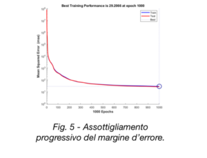
We asked to the ANN to find a way to generete a curve identical to a given curve, starting from the same inputs.
If you remember, we have to find a way to generate overlapping curves to the curves generated by the .-tir file, combining all the variables we have.
The first step is to feed the machine learning process, so we have to give to the ANN some inputs and outputs to process and compare.
We generate these input-output matrixes on a virtual “test bench” in Mathlab – the traditional way, let’s say…
We manually produce a limited number of tests to produce a performance curve of the tyre, in order to allow the ANN to learn (fig.6).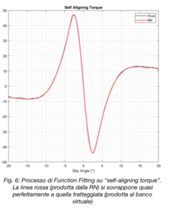
The big advantage the AI gives us is that once the ANN has learned, it doesn’t make the calculation process anytime (like Mathlab does), but it uses “shortcuts” that the ANN has created and tested to be reasonably affordable, with a limited margin of error.
At the end, it’s very similar to football: you can describe the process to reach the goal, describing the trajectory of the ball in every instant of the action, with a incredible high number of equations; or you can teach to your team a scheme or strategy to apply to the situation. Once you have decided the better scheme, you train the team: they repeat the scheme several times, till they execute it with enough precision. At this point the team is ready for a real match.
REAL-VIRTUAL COMPARISON
At the end of the process we have a .tir file from the real tyre, that generates some performance curves and we have a ANN ready to process a Function Fitting Process on this curves, after have learned on the test curves we generated on the virtual bench.
When the ANN generated curves overlap to the .tir generated ones, we’ve made it! We finally know all the characteristics to apply to our virtual tyre model. We fill the tyre model of the simulation environment with the data that the ANN finds and we are sure that our virtual tyre will behave exactly as the real one (or with a very little margin of error).
NEXT STEPS
Nowadays Skydrive’s ANN are ready to understand and replicate the physical and dynamical behave of the tyre. We did not consider the thermal component of the tyre, in order to see the number of variables low. As we said, any time we add a variable, we have to rise to one power the number of tests needed and the thermal component will add a big number of new variables.
Next step: implement the thermal component variables.
Not easy, but worth trying.